Demo

Usage · Encode

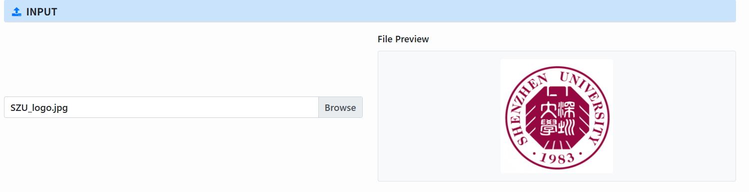
1. Select file (Input): Click Select file to choose the source file to encode (text/image/video, etc.). A preview appears at the right (image/video/text first 30 lines).
   
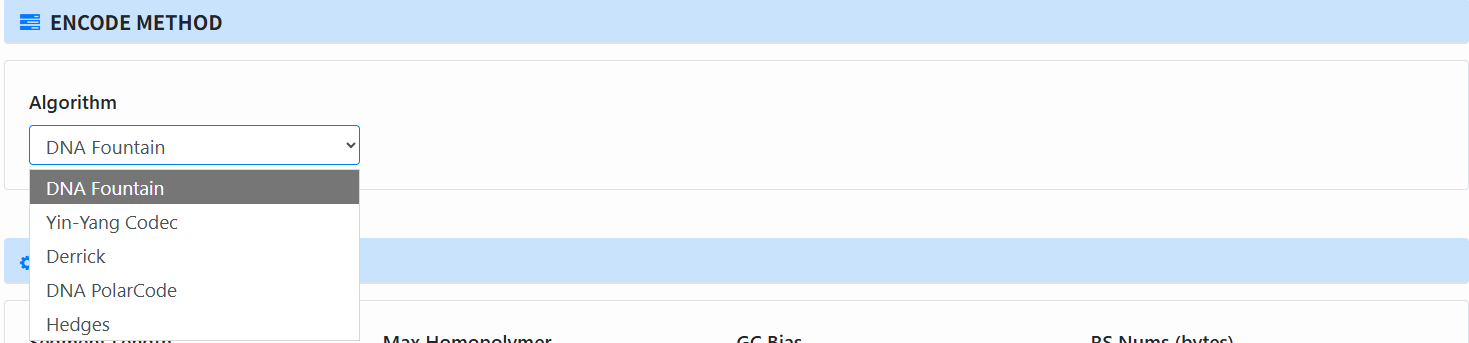
2. Select algorithm (Encode Method → Algorithm): Choose from DNA Fountain / Yin–Yang Codec / Derrick / PolarCode / Hedges.
   
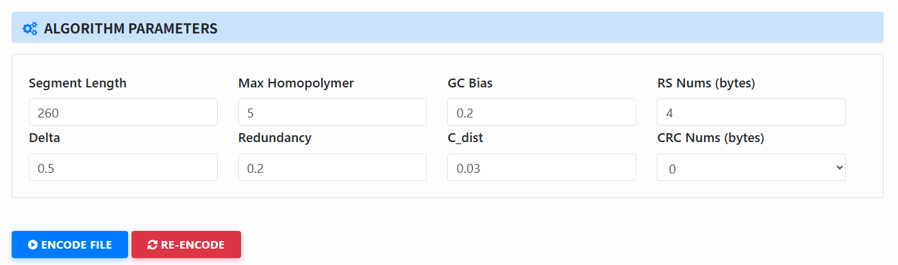
3. Fill in parameters (Algorithm Parameters): The page will show the parameter block for the selected algorithm (only parameters relevant to this algorithm appear). Adjust as needed.
   
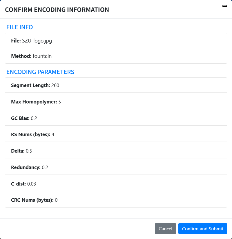
4. Start encoding: Click Encode File... A modal will pop up asking you to confirm the chosen settings. Verify and click Confirm and Submit.
   
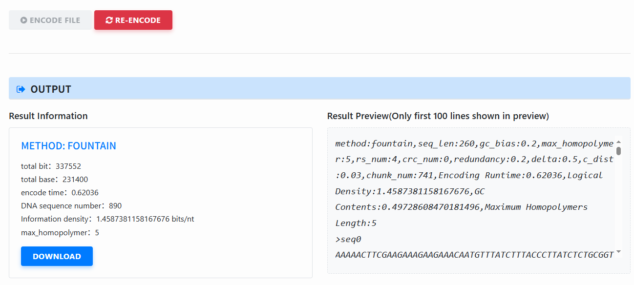
5. View results (Output): After encoding, a result panel appears (method, total bits/bases, time, number of sequences, information density, max homopolymer length, etc.). Click download to download the encoded FASTA.
   
6. Re-encode: Click Re-encode (right-side button) to reset the page, then change parameters or file and encode again.
   

Usage · Simulate

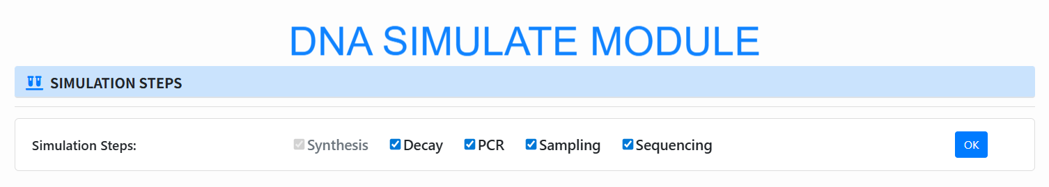
1. Choose pipeline steps (Simulation Steps): Check the stages to simulate (Synthesis is always on; optional Decay / PCR / Sampling / Sequencing), then click OK.
   
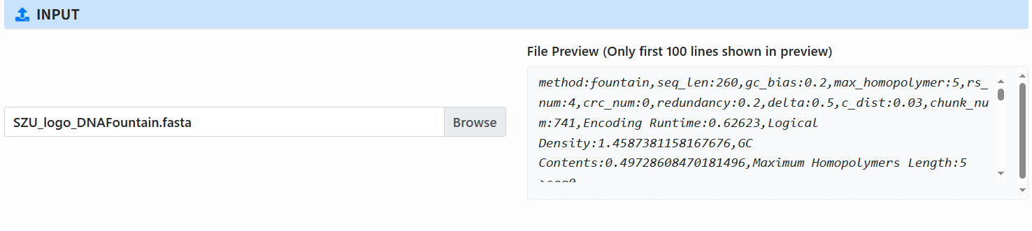
2. Select input file (Input): By default, use the FASTA/FA file from the previous Encode step; you can also select a new file (preview shows the first 100 lines).
   
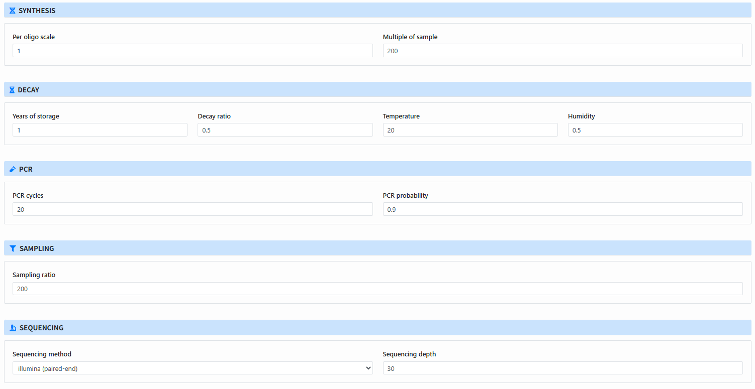
3. Configure parameters for each module: The page shows parameter blocks for selected steps:
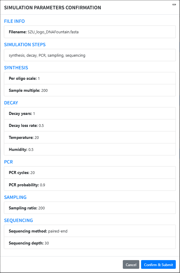
   • Synthesis: Per oligo scale, Multiple of sample
   • Decay: Years, Decay ratio, Temperature, Humidity
   • PCR: PCR cycles, PCR probability
   • Sampling: Sampling ratio
   • Sequencing: Sequencing method, Sequencing depth
   
4. Start simulation: Click start simulate (a confirmation modal appears). Verify File Info / Steps / Parameters and click Confirm & Submit to start the progress bar.
   
5. View & download results: After completion, see elapsed time in the result card and click download to get the generated sequencing files/results.
   
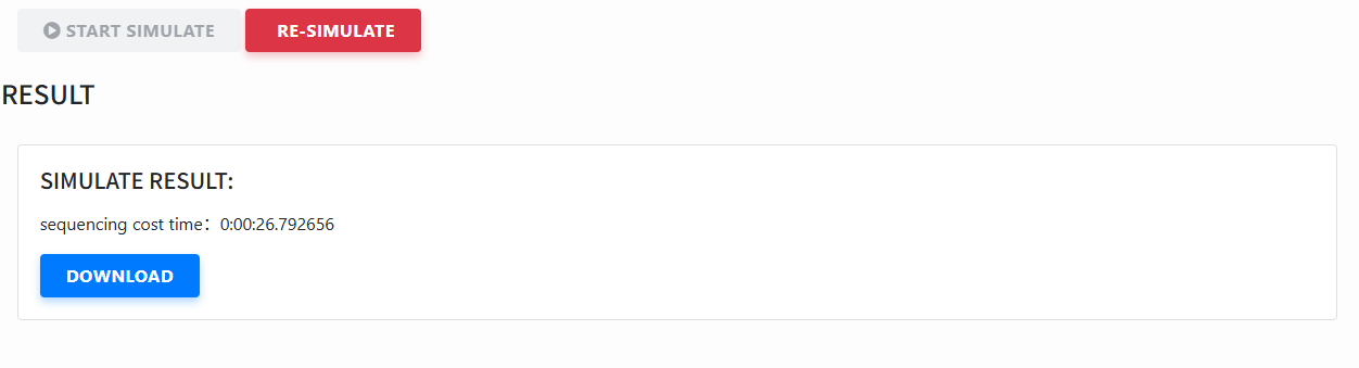
6. Re-simulate: Click Re-simulate to reset and run with different steps or parameters.

Usage · Decode

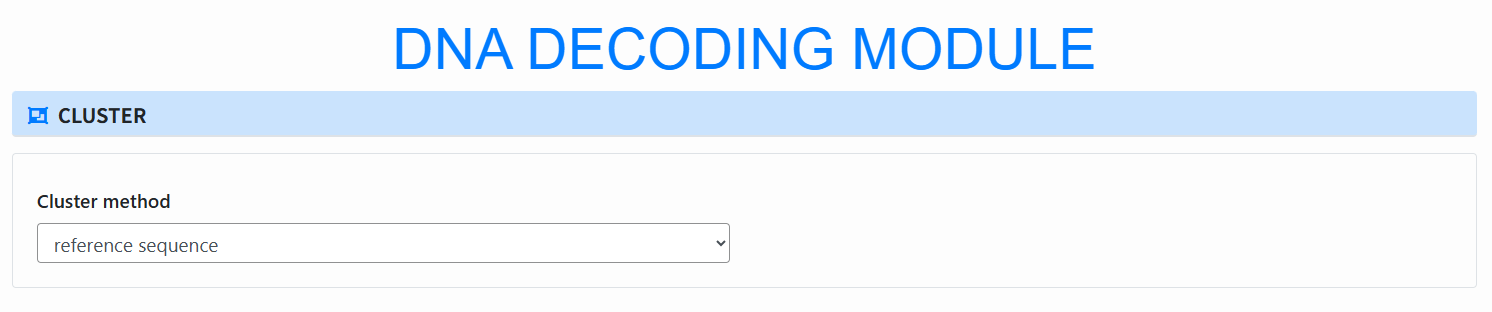
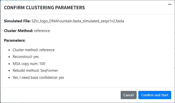
1. Select clustering method (Cluster): In the Cluster method dropdown choose:
   • index: index-based clustering (set Index length);
   • reference sequence: clustering via reference sequence; requires the Encode output (auto-filled if you encoded earlier);
   • I don't need cluster: skip clustering.
   • Note: if no simulation was run, you do not need clustering and reconstruction.
   
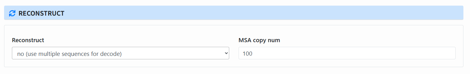
2. Set reconstruction parameters (Reconstruct):
   • Choose whether to use consensus for decoding (yes/no).
   • Set MSA copy num.
   • If reconstructing, choose Rebuild method (SeqFormer, bsalign, BMALA, DivBMA, Hybrid, Iterative, etc.).
   • Optional Base confidence (per-base confidence/quality for soft decoding).
   • Note: reconstruction uses MSA to recover the original encoded sequence from reads (Derrick always requires reconstruction).
   
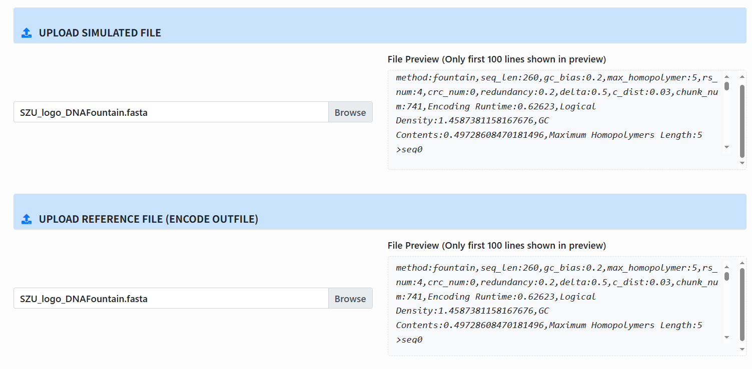
3. Upload files:
   • Simulated File: output from the simulation.
   • Reference File: the encoded reference file.
   Shows the first 100 lines.
   
4. Run clustering: Click Cluster Start, a confirmation dialog appears; confirm to run clustering.
   
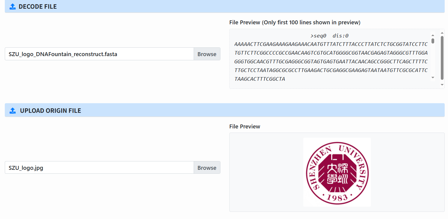
5. Upload files for decoding (enabled only after clustering completes):
   • Decode File: the clustering output.
   • Origin File: the original input file, used for final comparison.
   
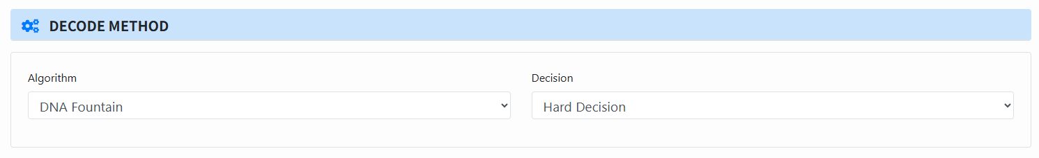
6. Select decoding method (Decode Method):
   • Algorithm: DNA Fountain, YYC, Derrick, Hedges.
   • Decision: choose Hard or Soft (Soft only when Reconstruct=yes and Base confidence=yes).
   
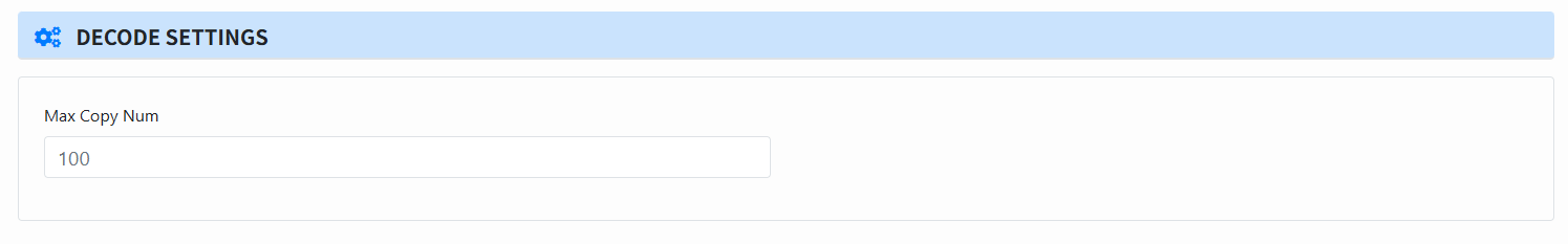
7. Set decoding parameters (Decode Settings):
   • Max Copy Num: number of sequences per cluster to use for decoding, which can only be used if no reconstruct is done
   Click Start Decode to open a confirmation dialog, verify parameters, and begin decoding.
   
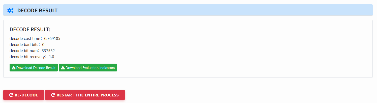
8. View decoding results:
   • Elapsed time, bad bits, total bits, recovery rate, etc.
   • Download Decode Result and Evaluation indicators (for the evaluate module).
   
9. Do it again:
   • Re-cluster: run clustering again.
   • Re-decode: run decoding again.
   • Restart the entire process: start over from the beginning.

Usage · Evaluate

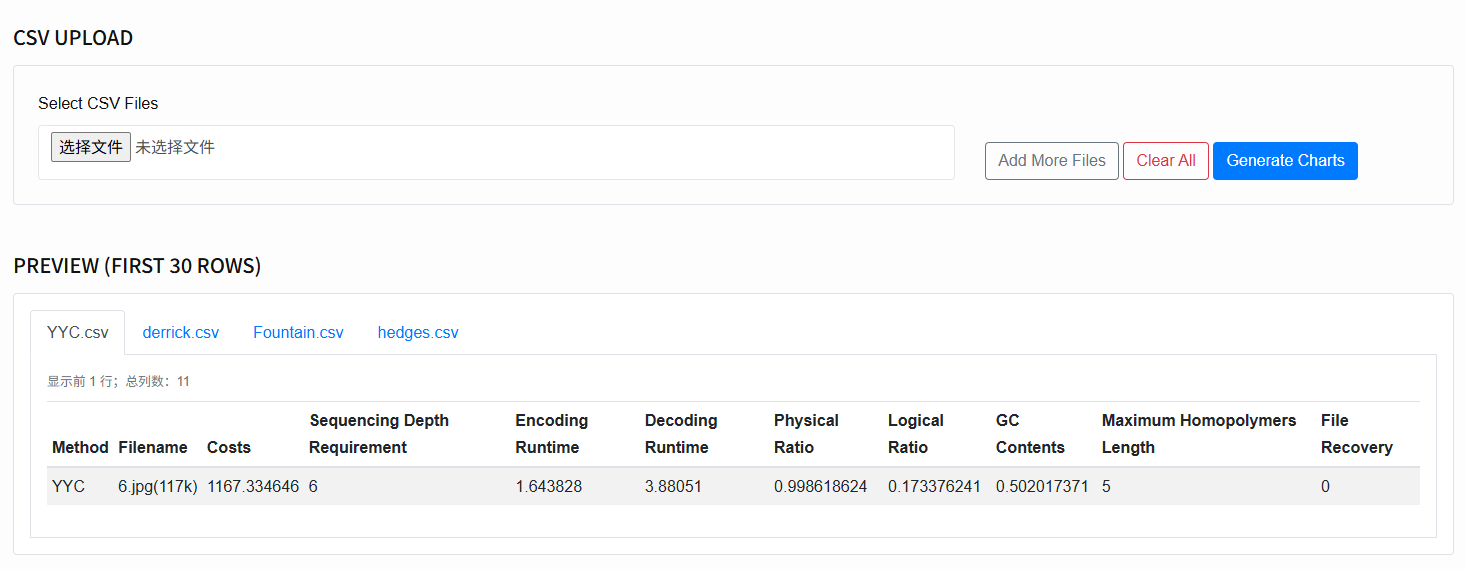
1. Upload CSV files: Each row represents one experiment or one method. Required columns (case-insensitive/aliases allowed): Method, Filename, and any of the following numeric columns: Costs, Sequencing Depth Requirement, Encoding Runtime, Decoding Runtime, Physical Ratio, Logical Ratio, GC Contents, Maximum Homopolymers Length, File Recovery.
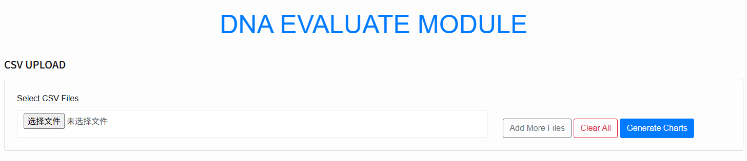
2. Select files (CSV Upload): Click Select CSV Files to choose one or more CSVs. To append, click Add More Files; to clear, click Clear All.
   
3. Preview: After selection, the system parses and shows the first 30 rows of each CSV so you can verify column names and formats.
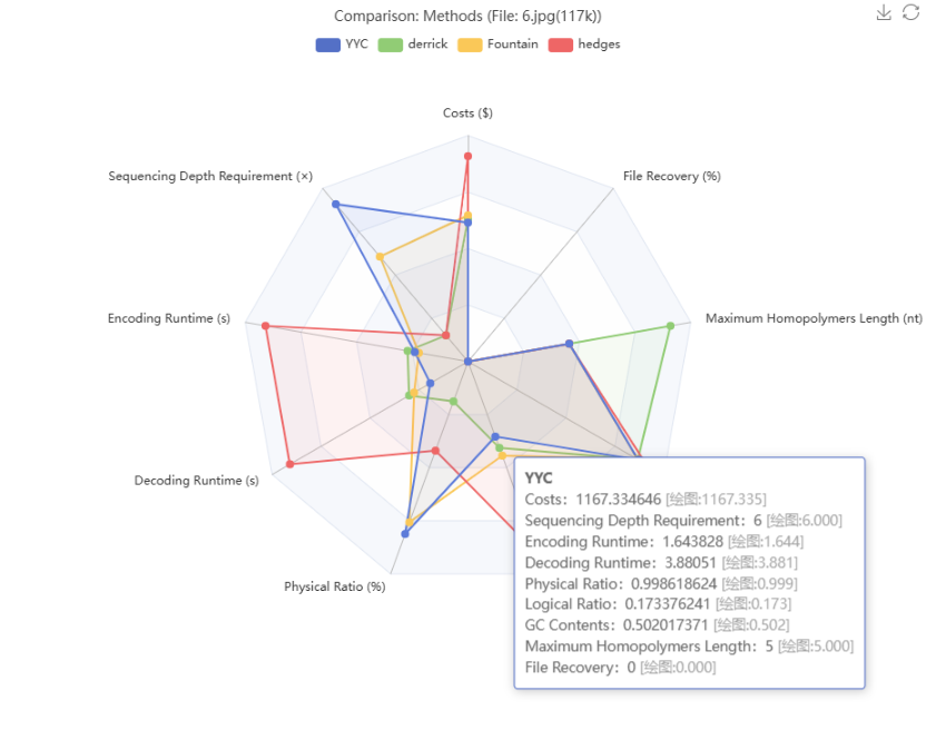
4. Evaluation mode: Two comparison modes are supported:
   • Same Method, Different Files — compare the same method across multiple files.
   • Same File, Different Methods — compare multiple methods on the same file.
   ⚠️ If both multiple methods and multiple files are detected simultaneously, the system prompts you to restrict to one dimension.
5. Generate charts: Click Generate Charts. The system merges valid data according to the chosen mode and renders a radar chart for performance comparison across methods or files.
   
6. Read the charts: Toggle methods/files via the legend; hover to view exact metric values. The tooltip displays both the raw mean and the normalized value used for plotting. Each metric is normalized against its own maximum to avoid scale bias.
   
7. Import again: When changing data, use Clear All to reset, or continue with Add More Files to add new files.
Tips:
• The two comparison modes are: (1) same file with different methods; (2) different files with the same method.
• You can zoom the radar chart with the mouse wheel.
• Hovering over a metric shows the original value.